Type I error and type II error: what are they and what do they indicate in statistics?

These concepts of statistics help us to understand how we can make mistakes with hypotheses.

When we do research in psychology, within inferential statistics we find two important concepts: type I error and type II error.. These arise when we are performing hypothesis testing with a null hypothesis and an alternative hypothesis.

In this article we will see exactly what they are, when we commit them, how we calculate them and how we can reduce them.

Parameter estimation methods

Inferential statistics is responsible for extracting or extrapolating conclusions from a population, based on information from a sample. That is, it allows us to describe certain variables that we want to study, at the population level.

Within it, we find parameter estimation methodsThe purpose of parameter estimation methods is to provide methods that allow us to determine (with a certain precision) the value of the parameters we want to analyze from a random sample of the population we are studying.

Parameter estimation can be of two types: point estimation (when a single value of the unknown parameter is estimated) and interval estimation (when a confidence interval is established where the unknown parameter would "fall"). It is within this second type, interval estimation, where we find the concepts we are analyzing today: type I error and type II error.

Type I error and type II error: what are they?

Type I error and type II error are types of errors that we can make when we are faced with the formulation of statistical hypotheses (such as the null hypothesis or the null hypothesis). (such as the null hypothesis or H0 and the alternative hypothesis or H1). That is, when we are performing hypothesis testing. But to understand these concepts, we must first contextualize their use in interval estimation.

As we have seen, interval estimation is based on a critical region from the parameter of the null hypothesis (H0) that we posed, as well as on the confidence interval from the sample estimator.

In other words, the objective is to to establish a mathematical interval where the parameter we want to study would fall. To do this, a series of steps must be taken.

1. Hypothesis formulation

The first step is to formulate the null hypothesis and the alternative hypothesis, which, as we shall see, will lead us to the concepts of type I error and type II error.

1.1. Null hypothesis (H0)

The null hypothesis (H0) is the hypothesis put forward by the researcher, which he provisionally accepts as true. It can only be rejected through a process of falsification or refutation.

Normally, what is done is to state the absence of effect or the absence of differences (for example, it would be to state that: "There is no difference between cognitive therapy and behavior therapy in the treatment of anxiety").

1.2. Alternative hypothesis (H1)

The alternative hypothesis (H1), on the other hand, is intended to supplant or replace the null hypothesis. It usually states that there is a difference or effect (e.g., "There is a difference between cognitive therapy and behavior therapy in the treatment of anxiety").

2. Determination of the significance level or alpha (α).

The second step in interval estimation is to determine the significance level or alpha (α). determining the level of significance or alpha (α) level.. This is set by the researcher at the beginning of the process; it is the maximum probability of error that we accept in rejecting the null hypothesis.

It usually takes small values, such as 0.001, 0.01 or 0.05. In other words, it would be the "ceiling" or maximum error that we are willing to commit as researchers. When the significance level is 0.05 (5%), for example, the confidence level is 0.95 (95%), and the two add up to 1 (100%).

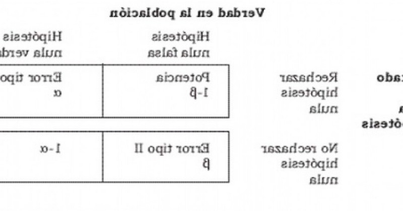
Once we establish the significance level, four situations can occur: that two types of errors occur (and this is where type I error and type II error come in), or that two types of correct decisions occur. That is to say, the four possibilities are:

2.1. Correct decision (1-α).

Consists of accepting the null hypothesis (H0) being true.. That is, we do not reject it, we maintain it, because it is true. Mathematically it would be calculated as follows: 1-α (where α is the type I error or significance level).

2.2. Correct decision (1-β)

In this case, we also make a correct decision; it consists of rejecting the null hypothesis (H0) being false. It is also called power of the test. It is calculated: 1-β (where β is the type II error).

2.3. Type I error (α)

The type I error, also called alpha (α), is made when rejecting the null hypothesis (H0) when it is true.. Thus, the probability of committing a type I error is α, which is the significance level we have set for our hypothesis test.

If for example the α we had set is 0.05, this would indicate that we are willing to accept a 5% probability of being wrong in rejecting the null hypothesis.

2.4. Type II error (β)

The type II error or beta (β), is committed when accepting the null hypothesis (H0) when it is false.. That is, the probability of making a type II error is beta (β), and depends on the power of the test (1-β).

To reduce the risk of making a type II error, we can choose to ensure that the test has sufficient power. To do this, we must ensure that the sample size is large enough to detect a difference when it actually exists.